RRTMG - The Rapid Radiative Transfer Model
Introduction
Treatment of Clouds
There are two methods in RRTMG, which handle clouds in different ways.
McICA
McICA allows us to have fractional cloud areas, by randomly assigning some wavelengths to see cloud and other wavelengths to see no cloud. For example if we have a cloud fraction of 40%, then 40% of the wavelengths see cloud, while the other 60% do not.
nomcica
With nomcica, all of the wavelengths see some cloud. Using this method for the shortwave we can only have cloud area fractions of zero and one, representing clear and completely overcast skies. On the other hand, if we are calculating longwave fluxes, we can also use fractional cloud area fractions.
Calculation of radiative fluxes
Longwave
Two properties are needed to calculate the longwave radiative fluxes; the absorptivity (or transmittance which equals one minus the absorptivity) and the emissivity. Values of these two properties are needed for each model layer, for both cloudy and clear sky regimes and for each waveband.
radld = radld * (1 - atrans(lev)) * (1 - efclfrac(lev,ib)) + &
        gassrc * (1 - cldfrac(lev)) + bbdtot * atot(lev) * cldfrac(lev)
The radiative fluxes at each layer(radld
on the left hand side of the equations) are calculated from the
radiative fluxes from the layer above (radld
on the right hand side of the equation) and the properties of
the layer.
The first term in the equation above is fraction of radiative
flux from the layer above that is transmitted through the layer.
atrans(lev) is the gaseous absorptivity and
efclfrac is the absorptivity of the cloud weighted by the
cloud area fraction (here for nomcica).
The other two terms in the above equation are emission terms.
The first of these represents emission from gases in the area of clear sky
and the second represents emission from gases and cloud from the area of cloud.
The equation for the upward longwave flux radlu is very similar: the flux
is calculated from the radiative flux from the layer below and the properties
of the layer.
These equations are used with nomcica when the rrtmg_cloud_overlap_method
is set to random and the cloud area fraction is greater
than 10-6. These calculations are in the rrtmg_lw_rtrn.f90 file,
in the downward radiative transfer loop and
upward radiative transfer loop respectively.
These equations are also used with McICA. In this case, efclfrac is either zero or the non-weighted
absorptivity of the cloud and this is allocated randomly to each waveband,
with the number of waveband receiving each depending on the cloud area fraction.
For McICA, these calculations are in the rrtmg_lw_rtrnmc.f90 file, in the
downward loop and upward loop respectively.
In both files, in the downward loop there are three different ways of calculating
the absorptivity, which use different approximations for the exponential of the
optical depth. The one that is used depends on the optical depth of the clear sky
and of the total sky.
With nomcica, if the rrtmg_cloud_overlap_method is set to any of the
other options except random, the rrtmg_lw_rtrnmr.f90 file
is called. Then, the radiative fluxes are calculated as follows, at the end of the
downward radiative transfer loop.
cldradd = cldradd * (1._rb - atot(lev)) + cldfrac(lev) * bbdtot * atot(lev)
clrradd = clrradd * (1._rb-atrans(lev)) + (1._rb - cldfrac(lev)) * gassrc
radld = cldradd + clrradd
The downward radiative flux is split into the clear sky and cloudy components,
clrradd and cldradd respectively.
Both components contain a transmittance term from the clear or cloudy part,
respectively, of the layer above and an emission term. The emission terms are
identical to those described above.
The fluxes clrradd and cldradd are modified by an amount that depends on the change in
cloud fraction between layers before they are used for the calculation of fluxes
in the layer below.
Clouds with McICA
A brief description of the different options that can be used in RRTMG with McICA and the input parameters required in each case.
Cloud properties
There are three options for the RRTMG inflag, as given in the climt dictionary: rrtmg_cloud_props_dict
  rrtmg_cloud_props_dict = {
      'direct_input': 0,
      'single_cloud_type': 1,
      'liquid_and_ice_clouds': 2
}
With McICA, we cannot use single_cloud_type, but can choose between direct_input and liquid_and_ice_clouds.
If we choose direct_input, we input the longwave_optical_thickness_due_to_cloud, shortwave_optical_thickness_due_to_cloud, as well as the shortwave parameters single_scattering_albedo_due_to_cloud, cloud_asymmetry_parameter and cloud_forward_scattering_fraction.
The cloud_forward_scattering_fraction is used to scale the other shortwave parameters (shortwave_optical_thickness_due_to_cloud, single_scattering_albedo_due_to_cloud and cloud_asymmetry_parameter), but it is not directly used in the radiative transfer calculations.
If the cloud_forward_scattering_fraction is set to zero, no scaling is applied.
The other cloud properties, namely cloud_ice_particle_size and cloud_water_droplet_radius, mass_content_of_cloud_ice_in_atmosphere_layer, and mass_content_of_cloud_liquid_water_in_atmosphere_layer are completely unused.
The RRTMG iceflag and liqflag are irrelevant.
On the other hand, if we choose liquid_and_ice_clouds,
any input values for longwave_optical_thickness_due_to_cloud, shortwave_optical_thickness_due_to_cloud, single_scattering_albedo_due_to_cloud and cloud_asymmetry_parameter are irrelevant.
Instead, these parameters are calculated from the cloud ice and water droplet particle sizes (cloud_ice_particle_size and cloud_water_droplet_radius), as well as the cloud ice and water paths (mass_content_of_cloud_ice_in_atmosphere_layer, mass_content_of_cloud_liquid_water_in_atmosphere_layer).
The methods used for the calculations depend on the cloud ice and water properties; iceflag and liqflag in RRTMG.
Regardless of the other cloud input type, cloud_area_fraction_in_atmosphere_layer is required,
and is used in McICA to determine how much of the wavelength spectrum sees cloud and how much does not.
Calculation of cloud properties
Longwave
For the longwave, the only cloud property of interest for calculating radiative fluxes in RRTMG, is the optical depth. This is calculated at the end of the longwave cldprmc submodule as:
taucmc(ig,lay) = ciwpmc(ig,lay) * abscoice(ig) + &
                 clwpmc(ig,lay) * abscoliq(ig)
Values of cloud optical depth taucmc are calculated for each model layer (pressure), lay, and each g-interval, ig.
The cloud ice and liquid absorption coefficients (abscoice and abscoliq) are multiplied by the cloud ice and liquid water paths (ciwpmc and clwpmc) respectively, to give the ice cloud optical depth and the liquid water cloud optical depth.
The cloud ice and liquid water paths are input by the user, in climt as mass_content_of_cloud_ice_in_atmosphere_layer and mass_content_of_cloud_liquid_water_in_atmosphere_layer respectively.
The cloud ice and liquid absorption coefficients are calculated based on the ice and liquid water particle sizes (specified by the user), and this calculation depends on the choice of iceflag and liqflag.
Shortwave
For the shortwave, there are three cloud properties, which affect the radiative flux calculation in RRTMG, namely the optical depth, the single scattering albedo and the asymmetry parameter.
The shortwave optical depth is calculated as:
taucmc(ig,lay) = tauice + tauliq
with
tauice = (1 - forwice(ig) + ssacoice(ig)) * ciwpmc(ig,lay) * extcoice(ig)
tauliq = (1 - forwliq(ig) + ssacoliq(ig)) * clwpmc(ig,lay) * extcoliq(ig)
The single scattering albedo is calculated as:
ssacmc(ig,lay) = (scatice + scatliq) / taucmc(ig,lay)
with
scatice = ssacoice(ig) * (1._rb - forwice(ig)) / (1._rb - forwice(ig) * ssacoice(ig)) * tauice
scatliq = ssacoliq(ig) * (1._rb - forwliq(ig)) / (1._rb - forwliq(ig) * ssacoliq(ig)) * tauliq
The asymmetry parameter is given by:
asmcmc(ig,lay) = 1.0_rb / (scatliq + scatice) * ( &
                 scatliq * (gliq(ig) - forwliq(ig)) / (1.0_rb - forwliq(ig)) + &
                 scatice * (gice(ig) - forwice(ig)) / (1.0_rb - forwice(ig)) )
The original RRTMG code for these calculations is at the end of the shortwave cldprmc submodule.
Values of optical depth, single scattering albedo and asymmetry parameter are calculated for each model layer (pressure), lay, and each g-interval, ig. The cloud ice and liquid water paths (ciwpmc and clwpmc) are input by the user.
The other parameters (extcoice, extcoliq, ssacoice, ssacoliq, gice, gliq, forwice, forwliq) are calculated based on the ice and liquid water particle sizes and this calculation depends on the choice of iceflag and liqflag.
Cloud ice properties
There are four options for the RRTMG iceflag. These are given in the climt dictionary: rrtmg_cloud_ice_props_dict
rrtmg_cloud_ice_props_dict = {
    'ebert_curry_one': 0,
    'ebert_curry_two': 1,
    'key_streamer_manual': 2,
    'fu': 3
}
ebert_curry_one
For the longwave, ebert_curry_one gives an absorption coefficient of
abscoice = 0.005 + 1.0 / radice
Here, radice is the ice particle size and the absorption coefficient is the same for all wavebands.
ebert_curry_one should not be used for the shortwave component with McICA.
ebert_curry_two
ebert_curry_two is the default choice for cloud ice optical properties in climt.
In this case, the longwave absorption coefficient is calculated in the lw_cldprmc file as follows.
abscoice(ig) = absice1(1,ib) + absice1(2,ib)/radice
The absorption coefficient abscoice is a function of g-interval ig and is made up of two contributions.
The first of these absice1(1, ib) comes from a look up table and is given in [m2/ g].
ib provides an index for the look up table, based on the waveband of the g-interval.
absice1(2,ib) also comes from a look up table and is given in [microns m2/ g]. It is divided by radice, the cloud ice particle size, providing an ice particle size dependence of the absorption coefficient.
Although the syntax does not emphasise it, the absorption coefficient may also depend on model layer (pressure), as radice can have model layer dependence.
radice comes from the input property labeled cloud_ice_particle_size in climt.
The ice particle size dependent term is more important than the independent term (absice1(2,ib)/radice > absice1(1,ib)) at all wavebands for ice particle sizes less than 88 microns.
Using ebert_curry_two, the ice particle size must be in the range [13, 130] microns, and even for larger particle sizes (> 88), the ice particle size dependent term is more important than the independent term for four of the five wavebands.
For the shortwave, the parameters (required for the optical depth, single scattering albedo and asymmetry) are calculated in the sw_cldprmc file as follows.
extcoice(ig) = abari(icx) + bbari(icx)/radice
ssacoice(ig) = 1._rb - cbari(icx) - dbari(icx) * radice
gice(ig) = ebari(icx) + fbari(icx) * radice
forwice(ig) = gice(ig)*gice(ig)
abari, bbari, cbari, dbari, ebari and fbari are all look up tables, containing five values, which correspond to five different wavebands.
The choice of waveband is indicated by icx.
The particle size dependence comes from radice, so each parameter consists of both a size independent and a size dependent contribution.
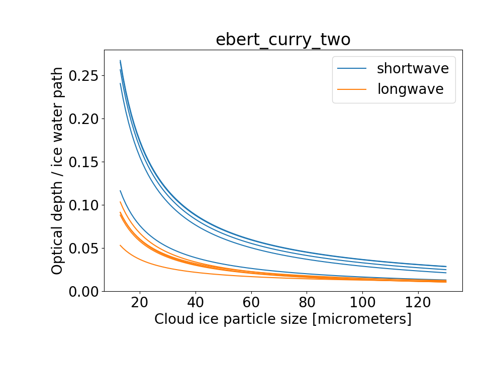
The dependence of cloud optical depth taucmc on cloud ice particle size (with an ice water path of 1), with different lines representing the different wavebands.
key_streamer_manual
In this case, both the longwave absorption coefficient and three of the shortwave parameters (excoice, ssacoice, gice) are interpolated from look up tables.
Comments in the RRTMG code state that these look up tables are for a spherical ice particle parameterisation.
The look up tables contain 42 values for each of the 16 longwave and 14 shortwave wavebands.
The 42 values correspond to different ice particle radii, evenly spaced in the range [5, 131] microns.
Ice particles must be within this range, otherwise an error is thrown.
The shortwave parameter forwice is calculated as the square of gice.
fu
The longwave absorption coefficient and shortwave parameters extcoice, ssacoice and gice are interpolated from look up tables.
The look up tables differ to those in key_streamer_manual, and
comments in the RRTMG code state that the look up tables for fu are for a hexagonal ice particle parameterisation.
The look up tables for fu are slightly larger than those for key_streamer_manual, and the range of allowed values for the ice particle size is corresponding larger ([5, 140] microns).
The shortwave parameter forwice is calculated from fdelta (again taken from look up tables) and ssacoice as follows.
forwice(ig) = fdelta(ig) + 0.5_rb / ssacoice(ig)
The longwave and shortwave parameter calculations can be found in the longwave cldprmc and shortwave cldprmc subroutines respectively.
Cloud liquid properties
There are two options for the RRTMG liqflag. These are given in the climt dictionary: rrtmg_cloud_liquid_props_dict
rrtmg_cloud_liquid_props_dict = {
    'radius_independent_absorption': 0,
    'radius_dependent_absorption': 1
}
For radius_independent_absorption, the longwave absorption coefficient is 0.0903614 for all wavebands.
This option should not be used for the shortwave.
radius_dependent_absorption is the default choice for cloud liquid water properties in climt.
In this case, the longwave absorption coefficient and the shortwave parameters extcoliq, ssacoliq, and gliq are interpolated from look up tables.
The look up tables have values for particle sizes in the range [2.5, 59.5] microns in 1 micron intervals (58 values) for each of the 16 longwave and 14 shortwave wavebands.
The shortwave parameter forwliq is calculated as the square of gliq.
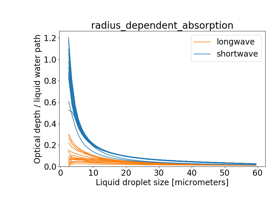
The dependence of cloud optical depth taucmc on cloud liquid water particle size (with a liquid water path of 1), with different lines representing the different wavebands.
Cloud overlap method
This is the RRTMG icld and is given in the climt dictionary: rrtmg_cloud_overlap_method_dict
rrtmg_cloud_overlap_method_dict = {
    'clear_only': 0,
    'random': 1,
    'maximum_random': 2,
    'maximum': 3
}
If we choose clear_only, there are no clouds, regardless of the other input.
If we choose random, the g-intervals which see cloud are chosen randomly for
each model layer. This means that there is a dependence on vertical resolution:
if vertical resolution is increased, more layers contain the same cloud
and a larger portion of the wavelength spectrum sees some of the cloud.
With maximum_random, the g-intervals that see cloud in one model layer are
the same as those that see cloud in a neighbouring model layer.
This maximises the cloud overlap between neighbouring layers (within a single
cloud). If the cloud area fraction changes between layers, the additional
g-intervals that see (or don’t see) cloud are assigned randomly. Therefore, if
there are two clouds at different altitudes, separated by clear sky, the two
clouds overlap randomly with respect to each other. If maximum is selected,
cloud overlap is maximised both within and between clouds.
The implementation is in the mcica_subcol_gen_sw and mcica_subcol_gen_lw
files, and consists firstly of assigning each g-interval a random number in the
range [0, 1]. For random, and maximum_random (cases 1 and 2 in
mcica_subcol_gen_sw and mcica_subcol_gen_lw), random numbers are generated
for each layer, whereas for maximum (case 3) only one set of random numbers
is generated and applied to all the layers. For maximum_random, the random
numbers are recalculated to fulfill the assumption about overlap (this
recalculation is described below).
Whether a g-interval at a certain layer sees cloud depends on both the random
number it has been assigned and the cloud fraction at that layer. For example,
if the cloud area fraction is 30%, all g-intervals that have been assigned a
random number > 0.7 (approximately 30% of the g-intervals) will see cloud.
The other g-intervals will see clear-sky. If the cloud fraction is 20%, only
g-intervals with a random number > 0.8 will see cloud.
The recalculation of random numbers in the maximum_random case for a certain
model layer (layer 2), considers the assigned random numbers and cloud area
fraction of the layer above (layer 1).
If the g-interval sees cloud in layer 1, its random number in layer 2 is
changed so that it matches that in layer 1. This does not necessarily mean that
it will see cloud in layer 2, because the cloud fraction could be smaller in
layer 2 than layer 1 (so the requirement for seeing cloud would be increased).
The random numbers for the g-intervals in layer 2, which do not see cloud in
layer 1, are multiplied by one minus the cloud area fraction of layer 1, so that
the set of random numbers assigned to layer 2 are still randomly distributed in
the range [0, 1]. This is required so that the right proportion of g-intervals
in layer 2 see cloud.
Differences in cloud input with nomcica
Regarding the options that can be used with nomcica, there are a few differences to those that can be used with McICA.
Cloud properties
For the longwave, we can choose single_cloud_type in the rrtmg_cloud_props_dict.
The longwave cloud optical depth is calculated as follows.
taucloud(lay,ib) = abscld1 * (ciwp(lay) + clwp(lay))
This gives us a cloud optical depth based on a single constant value, abscld1
and the total cloud water path.
Thus, for this option, the mass_content_of_cloud_ice_in_atmosphere_layer, and
mass_content_of_cloud_liquid_water_in_atmosphere_layer are needed as input.
single_cloud_type is not available for the shortwave.
If we choose liquid_and_ice_clouds, the calculations of the longwave and shortwave
optical properties from the cloud mass and particle sizes are the same as for McICA,
but are calculated for each waveband instead of each g-interval.
Cloud overlap method
With nomcica choosing a cloud overlap of random in the
rrtmg_cloud_overlap_method_dict is different to choosing either
maximum_random or maximum. The latter two options do not differ.
If we choose random, the radiative flux transmitted from one layer to the next
does not care if it came from cloud or clear sky,
whereas with maximum_random, the cloudy and clear fluxes are separated and
treated separately from one model layer to the next.